Fairbanks Weather Web Tracking

climate
R
temperature
nginx
Published

January 28, 2024

Introduction

Clouds roll in

Whenever it’s cold like it has been for the past week, the subject of my Local Fairbanks Temperatures page comes up in various places. Folks on Facebook were curious about how much traffic the page sees, so I thought I’d take a quick look. I don’t keep web server logs longer than two weeks and I don’t use Google Analytics or any of those other services because I don’t really care all that much how much “engagement” I’m getting or whether my “SEO” is good or not.

The first step is to figure out how to analyze the logs in the first place. I tried using a couple of the standard packages that are available, but something about my configuration was different than what they were expecting.

So I did it myself. It starts with a regular expression that pulls apart the bits and delimits them with the pipe character (|), which is unlikley to be found normally in the log files. Then I use the tidyr::separate function to split the delimited string into columns, do a bit of fiddling to correct the timestamp, identify the operating system of the clients, and pull out the request URL.

Code
library(tidyverse)
library(lubridate)

lines <- tibble(line = read_lines("local_weather.log"))
splitted <- lines |>
  mutate(
    splitted =
      gsub(
        '([^ ]+) ([^ ]+) - - \\[([^]]+)\\] "([^"]+)" ([0-9]+) ([0-9]+) "([^"]+)" "([^"]+)"',
        "\\1|\\2|\\3|\\4|\\5|\\6|\\7|\\8",
        line
      )
  ) |>
  separate_wider_delim(
    cols = splitted,
    names = c("host", "ip", "ts", "request", "response", "bytes", "referrer", "agent"),
    delim = "|",
    too_few = "align_start"
  ) |>
  mutate(
    ts = with_tz(dmy_hms(ts), tzone = "US/Alaska"),
    os = case_when(
      grepl("(iPhone|iPad)", agent) ~ "iOS",
      grepl("Android", agent) ~ "Android",
      grepl("(Macintosh|Darwin)", agent) ~ "MacOS",
      grepl("Linux", agent) ~ "Linux",
      grepl("Windows", agent) ~ "Windows",
      grepl("CrOS", agent) ~ "ChromeOS",
      grepl("facebook", agent) ~ "Facebook",
      TRUE ~ "Other"
    )
  ) |>
  separate_wider_delim(
    cols = request,
    names = c("get_post", "request_url", "protocol"),
    delim = " ",
    too_few = "align_start"
  ) |>
  select(-line)

Results

The results look like this for a single hit:

Code
splitted |>
  head(n = 1) |>
  glimpse()
Rows: 1
Columns: 11
$ host        <chr> "swingleydev.com"
$ ip          <chr> "66.223.139.211"
$ ts          <dttm> 2024-01-28 00:01:41
$ get_post    <chr> "GET"
$ request_url <chr> "/weather/local_weather.php"
$ protocol    <chr> "HTTP/1.1"
$ response    <chr> "200"
$ bytes       <chr> "2743"
$ referrer    <chr> "https://www.google.com/url?q=https://swingleydev.com/weat…
$ agent       <chr> "Mozilla/5.0 (iPhone; CPU iPhone OS 16_1 like Mac OS X) Ap…
$ os          <chr> "iOS"

At just after midnight, someone at an IP of 66.223.139.211 (a GCI address), hit the swingledev.com hostname (I’ve got several different ones that all point to the same site) after doing a Google search that yielded the Fairbanks Local Temperatures pages. They did this on an iPhone running iOS 16.1.

These are the sorts of details one can gather from the web server logs.

Throwing out the data from today (which isn’t over yet), here’s some of the things we can extract from this information.

Unique Visitors

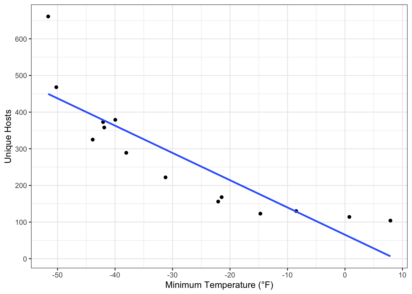
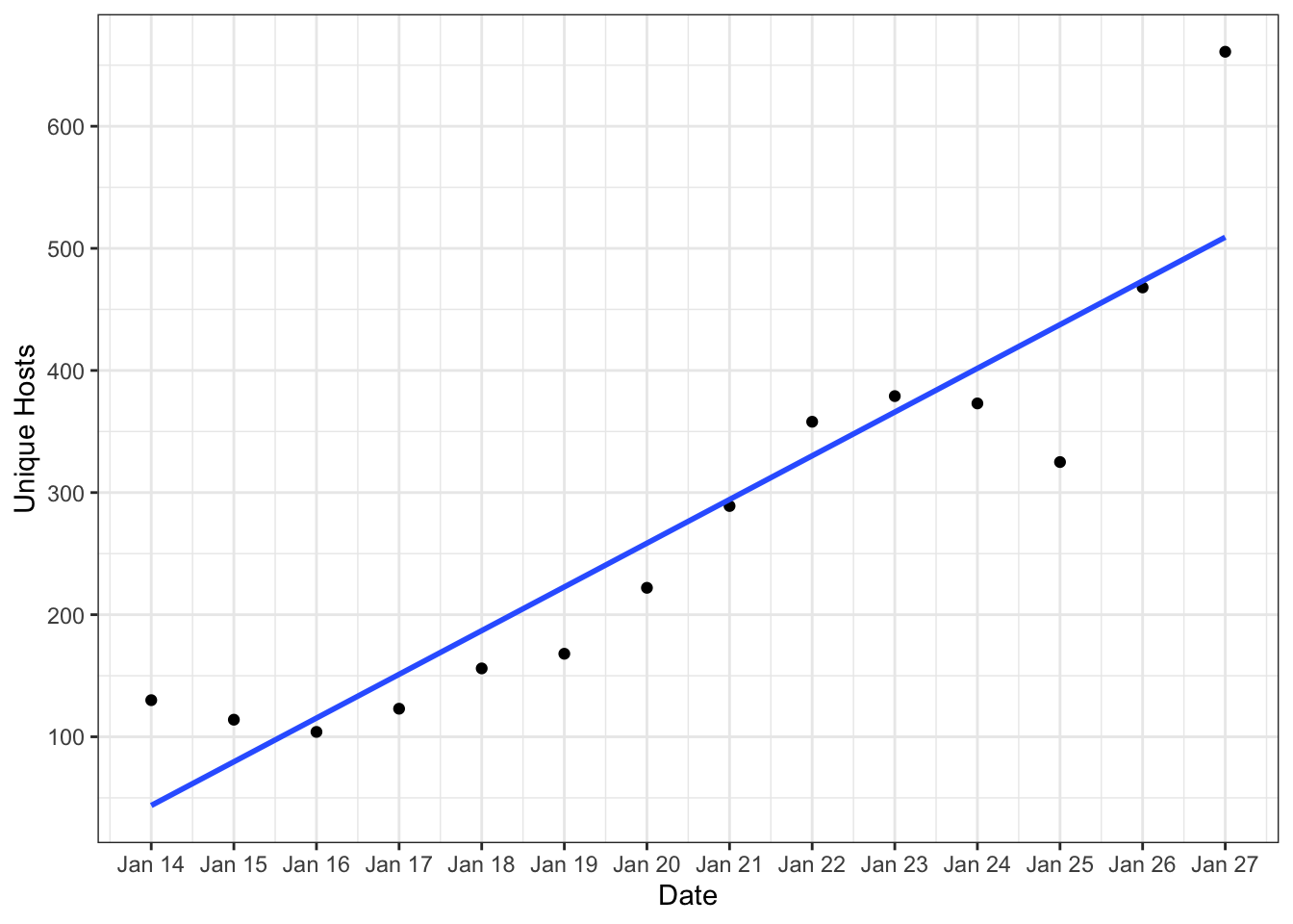
The number of different IP addresses that have loaded the page is a way of estimating how many different people have visited a site. We’ll remove the visitors using an unknown operating system, because those are probably web crawlers and not real people. I’m also adding a column for minimum daily temperature, since it has been suggested that more people visit the site when the temperatures are more extreme.

Code
library(gt)

hosts_by_day <- splitted |>
  filter(ts < today(), os != "Other") |>
  mutate(dte = date(ts)) |>
  group_by(dte, ip) |>
  summarize(.groups = "drop") |>
  count(dte) |>
  inner_join(min_temps, by = "dte") |>
  select(dte, min_temp, unique_hosts = n)

hosts_by_day |>
  gt() |>
  cols_label(
    dte = "Date",
    min_temp = "Minimum Temperature (°F)",
    unique_hosts = "Unique Visitors"
  ) |>
  cols_align(align = "left", columns = dte) |>
  fmt_number(
    decimals = 1,
    columns = min_temp
  )
Date Minimum Temperature (°F) Unique Visitors
2024-01-14 −8.5 130
2024-01-15 0.8 114
2024-01-16 7.9 104
2024-01-17 −14.7 123
2024-01-18 −22.1 156
2024-01-19 −21.5 168
2024-01-20 −31.2 222
2024-01-21 −38.0 289
2024-01-22 −41.9 358
2024-01-23 −40.0 379
2024-01-24 −42.1 373
2024-01-25 −43.9 325
2024-01-26 −50.2 468
2024-01-27 −51.6 661

Let’s assume a linear relationship between the number of visitors and the temperature:

Code
summary(lm(data = hosts_by_day, unique_hosts ~ min_temp))

Call:
lm(formula = unique_hosts ~ min_temp, data = hosts_by_day)

Residuals:
   Min     1Q Median     3Q    Max 
-75.73 -58.94 -12.30  25.73 211.40 

Coefficients:
            Estimate Std. Error t value  Pr(>|t|)    
(Intercept)   65.423     41.143   1.590     0.138    
min_temp      -7.441      1.219  -6.106 0.0000529 ***
---
Signif. codes:  0 '***' 0.001 '**' 0.01 '*' 0.05 '.' 0.1 ' ' 1

Residual standard error: 83.54 on 12 degrees of freedom
Multiple R-squared:  0.7565,    Adjusted R-squared:  0.7362 
F-statistic: 37.28 on 1 and 12 DF,  p-value: 0.00005289

Yes indeed, when it’s colder more folks are looking at the page. However, another explanation could be the site has become more popular over time since the temperatures started getting colder and the site has been mentioned more frequently on other sites. There’s also the problem that over the period of interest, the temperature has tended colder, making temperature and date related to one another.

Code
summary(lm(
  data = hosts_by_day,
  unique_hosts ~ dte + min_temp + dte * min_temp
))

Call:
lm(formula = unique_hosts ~ dte + min_temp + dte * min_temp, 
    data = hosts_by_day)

Residuals:
    Min      1Q  Median      3Q     Max 
-97.769  -8.406   0.714  15.801  85.371 

Coefficients:
                Estimate  Std. Error t value Pr(>|t|)   
(Intercept)  387373.6410 351082.8998   1.103   0.2957   
dte             -19.6205     17.7876  -1.103   0.2958   
min_temp      20013.1697   5730.5409   3.492   0.0058 **
dte:min_temp     -1.0141      0.2904  -3.492   0.0058 **
---
Signif. codes:  0 '***' 0.001 '**' 0.01 '*' 0.05 '.' 0.1 ' ' 1

Residual standard error: 48.51 on 10 degrees of freedom
Multiple R-squared:  0.9316,    Adjusted R-squared:  0.911 
F-statistic: 45.38 on 3 and 10 DF,  p-value: 0.000003943

When we include both date, minimum temperature, and the interaction between the two, date is no longer significant, so it appears that temperature is more likely the driving factor behind the popularity of the page.

Here’s what the individual relationships look like graphically.

Code
library(scales)
ggplot(data = hosts_by_day, aes(x = min_temp, y = unique_hosts)) +
  theme_bw() +
  geom_point() +
  geom_smooth(method = "lm", se = FALSE) +
  scale_x_continuous(
    name = "Minimum Temperature (°F)",
    breaks = pretty_breaks(n = 6)
  ) +
  scale_y_continuous(
    name = "Unique Hosts",
    breaks = pretty_breaks(n = 6)
  )
ggplot(data = hosts_by_day, aes(x = dte, y = unique_hosts)) +
  theme_bw() +
  geom_point() +
  geom_smooth(method = "lm", se = FALSE) +
  scale_x_date(
    name = "Date",
    date_breaks = "1 day",
    date_labels = "%b %d"
  ) +
  scale_y_continuous(
    name = "Unique Hosts",
    breaks = pretty_breaks(n = 6)
  )

Hosts by Temperature

Hosts by Date

Hits

In the early days of the Internet, site counters were a popular addition to a site so you could see how many hits a particular page received. It was a sort of thumbs up for your page that proved your page was valuable.

Here’s the daily data for that statistic, again, removing bots and web crawlers:

Code
hits_by_day <- splitted |>
  filter(ts < today(), os != "Other") |>
  mutate(dte = date(ts)) |>
  count(dte) |>
  inner_join(min_temps, by = "dte") |>
  select(dte, min_temp, hits = n)

hits_by_day |>
  gt() |>
  cols_label(
    dte = "Date",
    min_temp = "Minimum Temperature (°F)",
    hits = "Hits"
  ) |>
  cols_align(align = "left", columns = dte) |>
  fmt_number(
    decimals = 1,
    columns = min_temp
  )
Date Minimum Temperature (°F) Hits
2024-01-14 −8.5 222
2024-01-15 0.8 185
2024-01-16 7.9 189
2024-01-17 −14.7 226
2024-01-18 −22.1 305
2024-01-19 −21.5 349
2024-01-20 −31.2 598
2024-01-21 −38.0 786
2024-01-22 −41.9 902
2024-01-23 −40.0 902
2024-01-24 −42.1 828
2024-01-25 −43.9 849
2024-01-26 −50.2 1453
2024-01-27 −51.6 2219

And the regression:

Code
summary(lm(
  data = hits_by_day,
  hits ~ dte + min_temp + dte*min_temp
))

Call:
lm(formula = hits ~ dte + min_temp + dte * min_temp, data = hits_by_day)

Residuals:
    Min      1Q  Median      3Q     Max 
-360.36  -97.30   25.42   88.32  420.03 

Coefficients:
                Estimate  Std. Error t value Pr(>|t|)   
(Intercept)  1944615.756 1511875.708   1.286  0.22735   
dte              -98.513      76.599  -1.286  0.22739   
min_temp       85052.351   24677.549   3.447  0.00626 **
dte:min_temp      -4.309       1.250  -3.446  0.00626 **
---
Signif. codes:  0 '***' 0.001 '**' 0.01 '*' 0.05 '.' 0.1 ' ' 1

Residual standard error: 208.9 on 10 degrees of freedom
Multiple R-squared:  0.8977,    Adjusted R-squared:  0.8671 
F-statistic: 29.26 on 3 and 10 DF,  p-value: 0.00002895

Same pattern, but less predictive than with unique hosts.

Operating system

It’s always interesting to look at what sort of computers folks are using. Here’s the operating system, as identified by their user agent.

Code
splitted |>
  count(os) |>
  arrange(desc(n)) |>
  gt() |>
  cols_label(
    os = "Operating System",
    n = "Count"
  ) |>
  cols_align(align = "left", columns = os) |>
  fmt_number(
    decimals = 0,
    sep_mark = ","
  )
Operating System Count
iOS 4,906
Android 2,167
Windows 1,879
MacOS 1,165
Other 386
Facebook 301
Linux 171
ChromeOS 25

Most people (64%) are using mobile devices these days, and those are mostly iPhones or iPads (69% of mobile devices).